
Fitting a line: predictions, slope and R squared
On this page 6 headings
A fitted line summarizes an approximately linear pattern and lets us predict a numerical response from an explanatory value. Predictions can miss individual observations.
Read the equation before using it
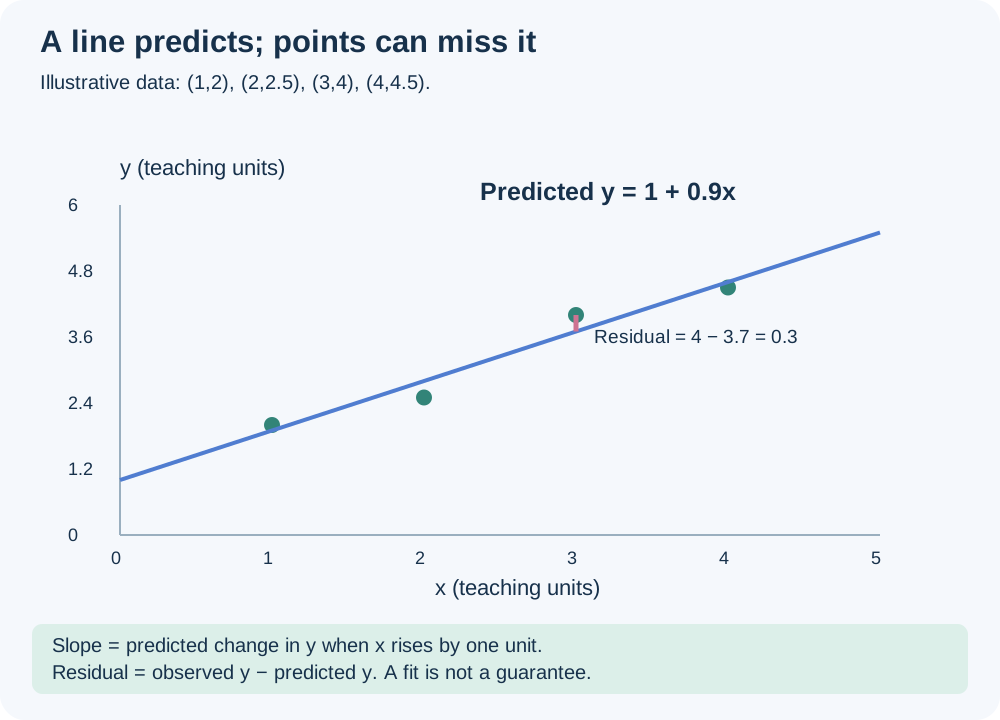
y-hat means predicted y. The intercept a is the predicted y when x = 0. The slope b is the predicted change in y for a one-unit increase in x. The units of slope are y-units per x-unit. An intercept can be mathematically necessary without being a sensible real-world prediction if x = 0 lies outside the data range.
How the line is chosen
The usual least-squares line minimizes the sum of squared vertical residuals. A residual is observed y minus predicted y. A positive residual means the observation is above the line; a negative residual means it is below.
These formulas add a way to check the fitted line by hand. They apply when x varies; if all x values are identical, a unique slope cannot be estimated.
Worked example: house size and price
The lecture gives the rounded line Predicted price = 36 + 30.5 × Size. Size is measured in thousands of square feet; price is in lakh rupees. An extra 1,000 sq ft is associated with about 30.5 lakh more predicted price.
| Size | Calculation using rounded lecture line | Predicted price |
|---|---|---|
| 2.0 (2,000 sq ft) | 36 + 30.5×2 | 97 lakh |
| 2.5 (2,500 sq ft) | 36 + 30.5×2.5 | 112.25 lakh |
| 3.0 (3,000 sq ft) | 36 + 30.5×3 | 127.5 lakh |
For the observed house at size 2.5 and price 98, the residual using this rounded line is 98−112.25 = −14.25 lakh. The actual house is priced below its prediction. Fitting the original 15 pairs at full precision gives slope ≈ 30.4807 and intercept ≈ 36.0188; small differences from the slide equation are rounding.
What R² tells us
For ordinary least-squares regression with one explanatory variable and an intercept, R² = r². It measures the fraction of variation in the observed response accounted for by the fitted line, relative to predicting the response mean. It does not mean that percentage of predictions are correct, and it does not measure causation.
| Lecture example | Rounded line | r | R² | Meaning |
|---|---|---|---|---|
| House example 1 | Price = 36 + 30.5×Size | ≈ +0.8045 | ≈ 0.647 | About 64.7% of observed price variation is accounted for by this line. |
| Car example | Price = 9.03 − 0.694×Age | ≈ −0.9247 | ≈ 0.855 | A strong negative fitted relationship. |
| House example 3 | Price = 130 + 7.77×Size | ≈ +0.149 | ≈ 0.022 | The line accounts for only about 2.2% of observed price variation. |
The latter two equations are separate lecture examples; do not combine them with the earlier five-car teaching data or assume the two housing lines fit the same dataset. R² has no sign, so use the slope or r to determine whether the relationship rises or falls.
A second complete calculation
For pairs (1,2),(2,2.5),(3,4),(4,4.5), x-bar = 2.5 and y-bar = 3.25. Sum of x squared deviations = 5; sum of products = 4.5. Slope = 4.5/5 = 0.9. Intercept = 3.25−0.9×2.5 = 1. Predicted y at x = 3 is 3.7; observed y is 4, so residual = 0.3.
Use a fit within its limits
Plot the data, check that a line is sensible, and inspect unusual points. Predicting within the observed x-range is interpolation. Predicting far outside it is extrapolation and may fail if the pattern changes. A line for sizes 0.8–3.4 thousand sq ft should not be trusted automatically for a 20-thousand-sq-ft house.
In a spreadsheet, fit a linear trendline to the scatterplot and display its equation and R². Read the units and retain enough decimal places for the required accuracy.
Try it yourself
A line is predicted cost = 100 + 20×distance, with distance in km. Interpret its slope.
Show explained answer
Each additional kilometer increases predicted cost by 20 currency units. The intercept is predicted cost at zero distance.
Try it yourself
If r = −0.8, what is R² for simple least squares with an intercept?
Show explained answer
0.64. About 64% of response variation is accounted for by the line. The relationship is negative even though R² is positive.
Try it yourself
Observed y is 12 and predicted y is 15. Find the residual.
Show explained answer
12−15 = −3. The point lies 3 y-units below the fitted line.
Source: Lectures 4.7 and 4.8. Extra examples and diagrams are teaching material prepared for these notes.