
Correlation: direction and strength without units
On this page 6 headings
Correlation standardizes covariance so its magnitude can be interpreted without measurement units. Pearson’s r summarizes a straight-line relationship.
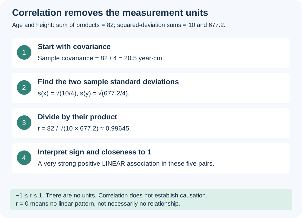
The sample n−1 factors cancel in the sums formula. If using covariance divided by standard deviations, use consistent sample definitions throughout, or consistent population definitions throughout. If either variable is constant, its SD is zero and correlation is undefined.
Read the sign and the absolute size
| r | Interpretation |
|---|---|
| +1 | Perfect positive straight-line relationship. |
| Near +1 | Strong positive linear association. |
| Near 0 | Little linear association; a curve may still exist. |
| Near −1 | Strong negative linear association. |
| −1 | Perfect negative straight-line relationship. |
There is no universal cutoff that makes every correlation “strong” in every subject. Interpret the magnitude alongside the scatterplot, sample size and context. Correlation has no units and lies between −1 and +1.
Worked example: age and height
For the five pairs, the sum of squared age deviations is 10, the sum of squared height deviations is 677.2, and the sum of paired products is 82.
This is a very strong positive linear relationship in these five observations. Keep full precision in intermediate values: using sample covariance 20.5, age SD √2.5 and height SD √169.3 gives the same result.
Worked example: car age and price
The car data have squared-deviation sums 10 and 10, and product sum −10. Thus r = −10/√(10×10) = −1. Every pair lies on Price = 7 − Age. This perfect example is a small teaching dataset, not a rule for all cars.
What changes r, and what does not?
Changing centimeters to meters, or adding the same constant to all measurements of one variable, leaves r unchanged. Multiplying just one variable by a negative number reverses the sign. Swapping x and y leaves r unchanged, although it changes a regression prediction problem. Outliers can strongly change r.
Zero correlation does not rule out a curve
For x = −2,−1,0,1,2 and y = 4,1,0,1,4, y equals x² exactly. The pattern is a perfect U-curve, but r = 0 because the negative and positive linear contributions cancel.
Spreadsheet and correlation matrix
For age in A2:A6 and height in B2:B6, =CORREL(A2:A6,B2:B6) calculates Pearson r. Keep rows paired and use the same complete cases. With several numerical variables, a correlation matrix lists r for every pair. It is symmetric, with 1 on the diagonal for nonconstant variables; it does not make a causal claim.
Try it yourself
Which is stronger as a linear association: r = −0.9 or r = +0.4?
Show explained answer
−0.9 has the stronger linear association because its absolute value is larger. The minus sign gives direction, not weakness.
Try it yourself
If r is 0.8 using kilograms, what is it after converting the same weights to grams?
Show explained answer
Still 0.8. Multiplying by a positive unit-conversion constant does not change correlation.
Try it yourself
Does r = 0.95 prove that x causes y?
Show explained answer
No. It describes strong linear association. Confounding, selection and other explanations remain possible.
Source: Lecture 4.7. Extra examples and diagrams are teaching material prepared for these notes.