
Row shares, column shares and association
On this page 6 headings
The phrase “out of whom?” decides the denominator. The share of women who own phones and the share of owners who are women are different quantities.
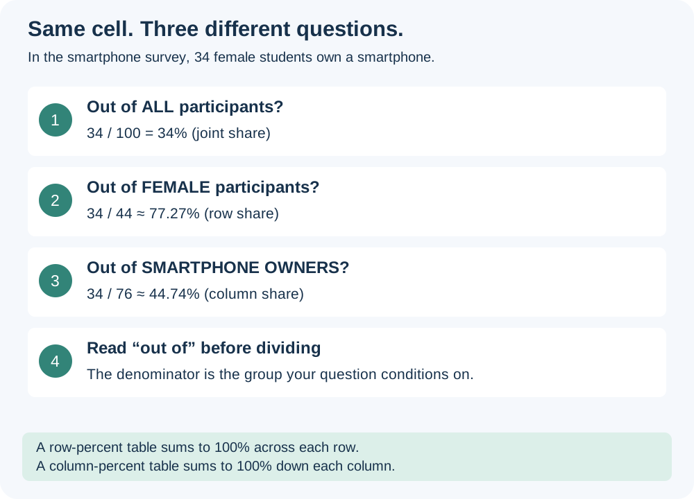
Overall, joint, row and column shares
| Question | Calculation | Result |
|---|---|---|
| What share of all participants own phones? | 76/100 | 76% (overall ownership share) |
| What share are female owners? | 34/100 | 34% (joint share) |
| Among female participants, what share own phones? | 34/44 | ≈ 77.27% (row share) |
| Among owners, what share are female? | 34/76 | ≈ 44.74% (column share) |
Row relative frequencies
Divide every cell in a row by its row total. The percentages across each row add to 100%, apart from rounding.
| Gender | No phone | Owns phone | Within-row total |
|---|---|---|---|
| Female | 10/44 ≈ 22.73% | 34/44 ≈ 77.27% | 100% |
| Male | 14/56 = 25% | 42/56 = 75% | 100% |
Column relative frequencies
Divide every cell in a column by its column total. The percentages down each column add to 100%.
| Gender | Among non-owners (n=24) | Among owners (n=76) |
|---|---|---|
| Female | 10/24 ≈ 41.67% | 34/76 ≈ 44.74% |
| Male | 14/24 ≈ 58.33% | 42/76 ≈ 55.26% |
| Within-column total | 100% | 100% |
Repeat for the income table
| Income | Ownership within income group | Share among all 62 owners | Share among all 38 non-owners |
|---|---|---|---|
| Low | 5/14 ≈ 35.71% | 5/62 ≈ 8.06% | 9/38 ≈ 23.68% |
| Medium | 39/66 ≈ 59.09% | 39/62 ≈ 62.90% | 27/38 ≈ 71.05% |
| High | 18/20 = 90% | 18/62 ≈ 29.03% | 2/38 ≈ 5.26% |
Association means one variable gives information about the other
If every row has exactly the same ownership distribution, knowing the row category gives no extra information about ownership in that table. The variables have no association in the empirical table. If the conditional distributions differ, there is association in the table. You can compare row profiles across rows or column profiles across columns; do not compare a row percentage with an unrelated column percentage.
The lecture describes the gender example as “not associated”, treating 77.27% and 75% as similar. They are close, but not exactly equal. Describe this as a small observed difference of about 2.27 percentage points. These notes do not use a significance test, so this sample alone does not establish exact independence in the population.
For income, the ownership shares differ much more: about 35.71%,59.09%,90%. In this sample, income group provides information about ownership. This is an observed association, not proof that changing income alone causes ownership.
Stacked counts versus 100% stacked shares
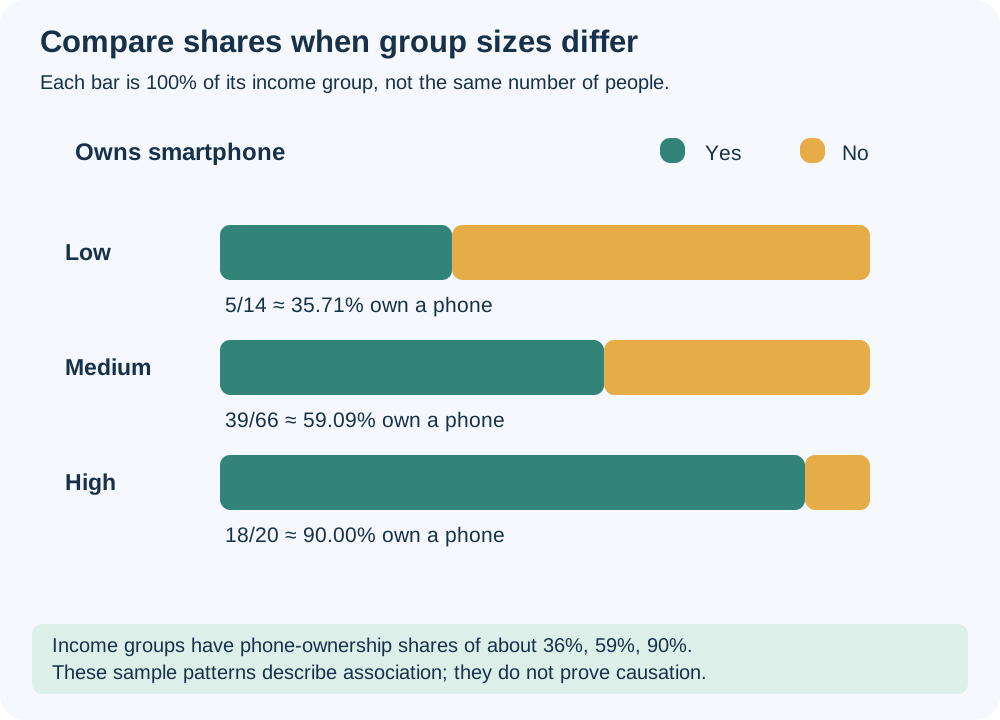
An ordinary stacked bar has total length equal to the group count, split into Yes and No counts. A 100% stacked bar gives each group the same total length and splits it into within-group shares. Use counts to show group sizes and 100% bars to compare compositions. Label the legend and denominator clearly.
Try it yourself
Which is the larger ownership share: 39 owners out of 66 medium-income participants, or 18 out of 20 high-income participants?
Show explained answer
High income: 18/20 = 90%, versus 39/66 ≈ 59.09%. The larger raw count was not the larger share.
Try it yourself
In a table with rows for board and columns for pass/fail, how do you find pass rate within each board?
Show explained answer
Divide the Pass cell in each board row by that board’s row total. Compare those row percentages.
Try it yourself
One group has 8 of 10 choosing A; another has 16 of 20. Are the profiles different?
Show explained answer
Both are 80% A and 20% not-A. The counts differ, but the conditional profiles match exactly.
Source: Lecture 4.3. Extra examples and diagrams are teaching material prepared for these notes.