
Numerical frequency tables: values and intervals
On this page 5 headings
A numerical variable records an amount, such as household size, height, or marks. Before finding an average, organize the numbers so you can see which values occur often.
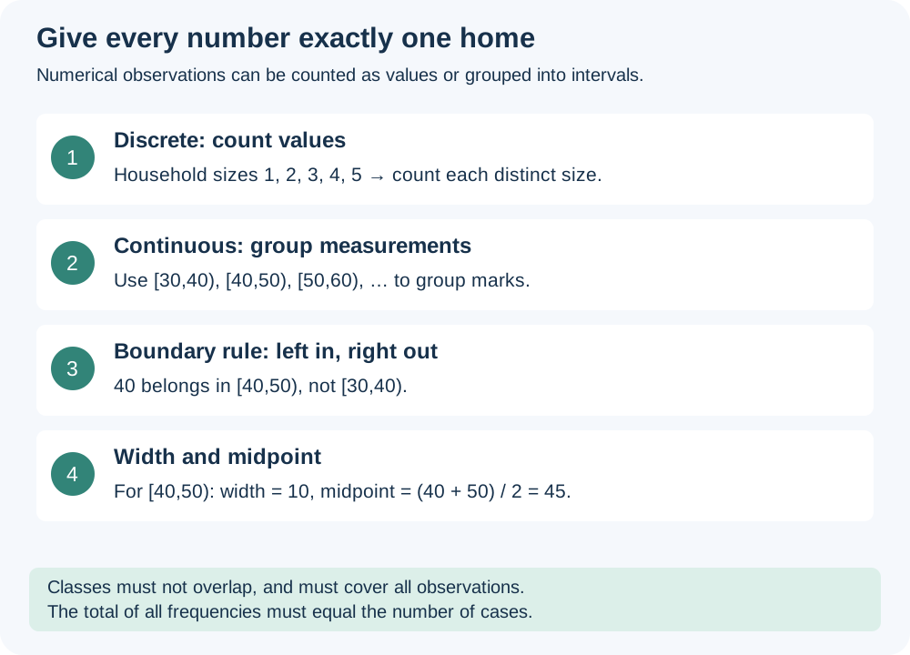
Discrete counts and continuous measurements
A discrete variable usually counts things: 1, 2 or 3 people in a household. A continuous variable usually measures things: height might be 162.4 cm. Recorded measurements are often rounded, but the quantity itself can still be continuous. Large sets of discrete values can also be grouped into intervals.
Worked example: household sizes
The lecture gives 15 responses: 2,1,3,4,5,2,3,3,3,4,4,1,2,3,4. List each distinct value, count it, then divide by 15 to find its relative frequency.
| People in household | Frequency | Relative frequency |
|---|---|---|
| 1 | 2 | 2/15 ≈ 0.1333 |
| 2 | 3 | 3/15 = 0.2 |
| 3 | 5 | 5/15 ≈ 0.3333 |
| 4 | 4 | 4/15 ≈ 0.2667 |
| 5 | 1 | 1/15 ≈ 0.0667 |
| Total | 15 | 1 |
Group many values into classes
A class, bin, or interval is a range of values. For example, [40,50) includes 40 and all values below 50, but excludes 50. The next class [50,60) includes 50. This left-in, right-out rule ensures that boundary values are counted once.
| Term | Meaning for [40,50) |
|---|---|
| Lower endpoint | 40, included |
| Upper endpoint | 50, excluded |
| Class width | 50 − 40 = 10 |
| Class mark / midpoint | (40 + 50)/2 = 45 |
For half-open continuous intervals there is no greatest included real number below 50. Think of 50 as the upper boundary, rather than an included maximum. If an exercise uses inclusive integer limits such as 40–49, read that convention carefully.
Worked example: the lecture’s grouped marks table
| Marks interval | Frequency | Relative frequency |
|---|---|---|
| [30,40) | 3 | 3/50 = 0.06 |
| [40,50) | 6 | 6/50 = 0.12 |
| [50,60) | 18 | 18/50 = 0.36 |
| [60,70) | 17 | 17/50 = 0.34 |
| [70,80) | 4 | 4/50 = 0.08 |
| [80,90) | 2 | 2/50 = 0.04 |
| Total | 50 | 1 |
Source clarification: the printed raw marks list contains 49 numbers, while the grouped table totals 50. Counting that printed list gives 17 in [50,60), not 18. Here we label the 50-case grouped table as given; we do not invent a missing observation. Use the stated grouped table when a question supplies it.
Choose sensible classes
The lecture suggests roughly 5–20 classes as a starting point, not a law. Too few bins hide detail; too many make the picture noisy. Cover every observation, avoid overlap, and normally use equal widths. Keep the bins in numerical order.
Try it yourself
Which class contains 60: [50,60) or [60,70)?
Show explained answer
[60,70). Its left endpoint is included; the earlier class excludes its right endpoint.
Try it yourself
Data are 1,2,2,3,3,3. Give the frequency and relative frequency for 3.
Show explained answer
Frequency = 3. Relative frequency = 3/6 = 0.5 = 50%.
Try it yourself
What is the midpoint of [20,30)?
Show explained answer
(20 + 30)/2 = 25. The midpoint is a representative value, not necessarily an observed value.
Source: Lecture 3.1. Extra examples and diagrams are teaching material prepared for these notes.