
Representing Graphs — Adjacency Matrix and Adjacency List
Start here Looking at a picture, we can "see" that one city is reachable from another. A computer can't see pictures. We must store the graph in a data structure. There are two standard ways: an adjacency matrix (a table of 0s and 1s) and an adjacency list (for each vertex, a list of its neighbours).
The example graph — airline routes
We use the lecture's airline graph all week: 10 cities numbered 0 to 9 (city 0 is Delhi and city 9 is Madurai in the lecture's story).
Directed version (one-way routes), 17 edges:
| From | To |
|---|---|
| 0 | 1, 4 |
| 1 | 2 |
| 2 | 0 |
| 3 | 4, 6 |
| 4 | 0, 3, 7 |
| 5 | 3, 7 |
| 6 | 5 |
| 7 | 4, 8 |
| 8 | 5, 9 |
| 9 | 8 |
Undirected version (all routes two-way), 13 edges: 0–1, 0–2, 0–4, 1–2, 3–4, 3–5, 3–6, 4–7, 5–6, 5–7, 5–8, 7–8, 8–9.
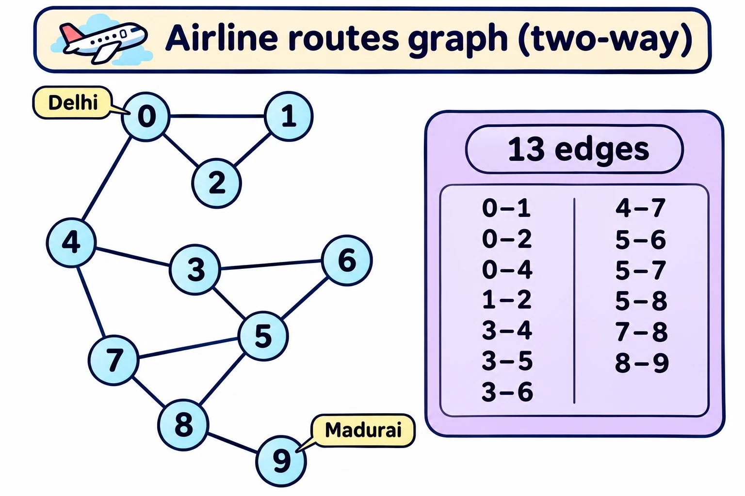
Naming vertices. We assume V = {0, 1, ..., n − 1}. If vertices have real names ("Delhi", "Madurai"), keep a small table mapping each name to a number. We also assume no self-loops (no edge from a vertex to itself).
1. Adjacency matrix
An n × n table A, with rows and columns numbered 0 to n − 1:
A[i, j] = 1 if (i, j) is an edge, else 0.
Directed airline graph:
| 0 | 1 | 2 | 3 | 4 | 5 | 6 | 7 | 8 | 9 | |
|---|---|---|---|---|---|---|---|---|---|---|
| 0 | 0 | 1 | 0 | 0 | 1 | 0 | 0 | 0 | 0 | 0 |
| 1 | 0 | 0 | 1 | 0 | 0 | 0 | 0 | 0 | 0 | 0 |
| 2 | 1 | 0 | 0 | 0 | 0 | 0 | 0 | 0 | 0 | 0 |
| 3 | 0 | 0 | 0 | 0 | 1 | 0 | 1 | 0 | 0 | 0 |
| 4 | 1 | 0 | 0 | 1 | 0 | 0 | 0 | 1 | 0 | 0 |
| 5 | 0 | 0 | 0 | 1 | 0 | 0 | 0 | 1 | 0 | 0 |
| 6 | 0 | 0 | 0 | 0 | 0 | 1 | 0 | 0 | 0 | 0 |
| 7 | 0 | 0 | 0 | 0 | 1 | 0 | 0 | 0 | 1 | 0 |
| 8 | 0 | 0 | 0 | 0 | 0 | 1 | 0 | 0 | 0 | 1 |
| 9 | 0 | 0 | 0 | 0 | 0 | 0 | 0 | 0 | 1 | 0 |
How to read it: row 4 has 1s in columns 0, 3 and 7 → edges 4 → 0, 4 → 3, 4 → 7.
- In a directed graph: row i = outgoing edges of i, column j = incoming edges of j.
- In an undirected graph: A[i, j] = A[j, i], so the matrix is symmetric across the main diagonal.
Undirected airline graph:
| 0 | 1 | 2 | 3 | 4 | 5 | 6 | 7 | 8 | 9 | |
|---|---|---|---|---|---|---|---|---|---|---|
| 0 | 0 | 1 | 1 | 0 | 1 | 0 | 0 | 0 | 0 | 0 |
| 1 | 1 | 0 | 1 | 0 | 0 | 0 | 0 | 0 | 0 | 0 |
| 2 | 1 | 1 | 0 | 0 | 0 | 0 | 0 | 0 | 0 | 0 |
| 3 | 0 | 0 | 0 | 0 | 1 | 1 | 1 | 0 | 0 | 0 |
| 4 | 1 | 0 | 0 | 1 | 0 | 0 | 0 | 1 | 0 | 0 |
| 5 | 0 | 0 | 0 | 1 | 0 | 0 | 1 | 1 | 1 | 0 |
| 6 | 0 | 0 | 0 | 1 | 0 | 1 | 0 | 0 | 0 | 0 |
| 7 | 0 | 0 | 0 | 0 | 1 | 1 | 0 | 0 | 1 | 0 |
| 8 | 0 | 0 | 0 | 0 | 0 | 1 | 0 | 1 | 0 | 1 |
| 9 | 0 | 0 | 0 | 0 | 0 | 0 | 0 | 0 | 1 | 0 |
Finding neighbours with the matrix
Scan row i; every column j with a 1 is a neighbour.
def neighbours(AMat, i):
    nbrs = []
    (rows, cols) = AMat.shape      # AMat is a NumPy array
    for j in range(cols):
        if AMat[i, j] == 1:
            nbrs.append(j)
    return nbrs
Undirected graph: neighbours(A, 7) → [4, 5, 8]; neighbours(A, 6) → [3, 5].
This always scans all n entries of the row, however few neighbours there are: O(n).
Degree
| Graph | Term | Meaning | How to find it in the matrix |
|---|---|---|---|
| Undirected | degree(i) | Number of edges touching i | Count the 1s in row i |
| Directed | outdegree(i) | Number of edges going out of i | Count the 1s in row i |
| Directed | indegree(i) | Number of edges coming into i | Count the 1s in column i |
Examples: undirected: degree(6) = 2 (neighbours 3 and 5). Directed: outdegree(6) = 1 (6 → 5) and indegree(6) = 1 (3 → 6).
Careful — a slide carry-over. On the directed-graph slides, the side note still says "Neighbours of 6 are [3, 5]". That is true for the undirected graph. In the directed graph, row 6 has a single 1, so 6 has only one outgoing neighbour: 5. (3 is an incoming neighbour: 3 → 6.)
2. Adjacency list
The matrix has n² entries no matter how many edges there are, and most of them are 0.
- Undirected graph: at most n(n − 1)/2 edges. Directed: at most n(n − 1).
- Real graphs usually have far fewer edges than n².
Adjacency list: for each vertex, store just the list of its neighbours. In Python, use a dictionary of lists:
AList = {}
for i in range(10):
    AList[i] = []
for (i, j) in edges:          # edges = list of (from, to) pairs
    AList[i].append(j)
print(AList)
Directed airline graph:
{0: [1, 4], 1: [2], 2: [0], 3: [4, 6], 4: [0, 3, 7],
 5: [3, 7], 6: [5], 7: [4, 8], 8: [5, 9], 9: [8]}
Undirected airline graph (each edge appears in both lists):
{0: [1, 2, 4], 1: [0, 2], 2: [0, 1], 3: [4, 5, 6], 4: [0, 3, 7],
 5: [3, 6, 7, 8], 6: [3, 5], 7: [4, 5, 8], 8: [5, 7, 9], 9: [8]}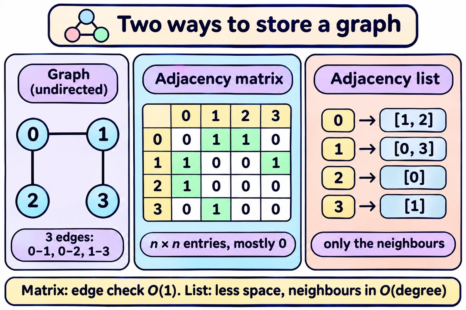
Comparing the two
| Question | Adjacency matrix | Adjacency list |
|---|---|---|
| Space needed | n² entries, always | About n + m (m = number of edges) — usually much less |
| Is j a neighbour of i? | Check A[i, j]: O(1) | Scan i's list: up to degree(i) steps |
| List all neighbours of i | Scan the whole row: O(n) | Read i's list: O(degree(i)) |
Choose the representation based on what your algorithm does most. Exploring graphs (BFS, DFS) mostly asks "give me all neighbours", so adjacency lists are usually better.
Checking reachability — the idea
Is Delhi (0) reachable from Madurai (9)?
- Mark 9 as reachable.
- Mark each neighbour of 9 as reachable.
- Keep going: systematically mark neighbours of marked vertices.
- Stop when 0 gets marked — reachable. If the marking stops spreading and 0 is still unmarked — unreachable.
We need a systematic order for exploring. Two main strategies:
- Breadth first (BFS): spread the marks in layers — next page.
- Depth first (DFS): follow one path as far as it goes, then backtrack.
In one line: Store a graph as an adjacency matrix (n × n table of 0/1, O(1) edge check, O(n) to list neighbours) or an adjacency list (dictionary of neighbour lists, less space, O(degree) to list neighbours).
Exam words: adjacency matrix, symmetric, adjacency list, dictionary of lists, neighbours, degree, indegree, outdegree, self-loop, n and m, sparse graph.