
Applications of BFS and DFS
Start here BFS and DFS answer "what can I reach?". But they can tell us much more about a graph: how many separate pieces it has, whether it contains a cycle, and (in directed graphs) which groups of vertices can all reach each other. The key tool is DFS numbering — recording when DFS enters and leaves each vertex.
Quick recap
- BFS works level by level and finds shortest paths (in number of edges).
- DFS dives deep, suspending each vertex while it explores its neighbours.
- DFS numbering records the order in which DFS explores vertices.
1. Connected components (undirected graphs)
An undirected graph is connected if every vertex is reachable from every other vertex.
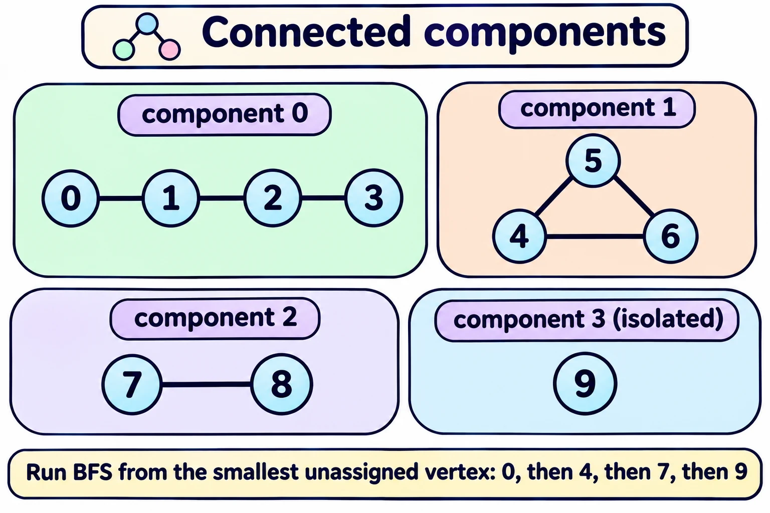
If it isn't connected, it splits into connected components: maximal groups of vertices that are connected among themselves. A vertex with no edges at all (an isolated vertex) is a component on its own.
Method:
- Start BFS (or DFS) from vertex 0. Every vertex it visits gets component number 0.
- Pick the smallest vertex not yet assigned a component. Run BFS from it; give everything it visits component number 1.
- Repeat until every vertex has a component number.
def Components(AList):
    component = {}
    for i in AList.keys():
        component[i] = -1
    (compid, seen) = (0, 0)
    while seen <= max(AList.keys()):
        startv = min([i for i in AList.keys() if component[i] == -1])
        visited = BFSList(AList, startv)
        for i in visited.keys():
            if visited[i]:
                seen = seen + 1
                component[i] = compid
        compid = compid + 1
return component(seen counts how many vertices have been assigned so far. With vertices 0 to n − 1, the loop stops once all n are seen.)
Worked example. 10 vertices; edges 0–1, 1–2, 2–3, 4–5, 5–6, 4–6, 7–8; vertex 9 has no edges.
| BFS started from | Vertices reached | Component number |
|---|---|---|
| 0 | 0, 1, 2, 3 | 0 |
| 4 (smallest unassigned) | 4, 5, 6 | 1 |
| 7 | 7, 8 | 2 |
| 9 | 9 (isolated) | 3 |
Result (we ran it): {0: 0, 1: 0, 2: 0, 3: 0, 4: 1, 5: 1, 6: 1, 7: 2, 8: 2, 9: 3} → 4 components.
2. Detecting cycles (undirected graphs)
A cycle is a path that starts and ends at the same vertex, without repeating an edge.
- Going i – j – i is not a cycle (it reuses the same edge back).
- A simple cycle repeats only the start/end vertex.
- A graph with no cycles is acyclic.
BFS tree and DFS tree
The edges that BFS uses to discover new vertices (k discovered from j → edge j–k) form a tree. (Technically one tree per component; several trees together are called a forest.)
Any edge that is NOT a tree edge creates a cycle. So: run BFS or DFS; if you find a non-tree edge, the graph has a cycle.
Example. A square: edges 0–1, 0–2, 1–3, 2–3. BFS from 0:
- Explore 0 → discover 1 and 2 (tree edges 0–1, 0–2).
- Explore 1 → discover 3 (tree edge 1–3).
- Explore 2 → its neighbour 3 is already visited, and 3 is not 2's parent. Edge 2–3 is a non-tree edge → cycle! (0 – 1 – 3 – 2 – 0.)
3. DFS numbering — pre and post
Keep a counter, starting at 0. Increase it every time DFS starts exploring a vertex and every time it finishes one.
- pre[v] = counter value when DFS enters v (entry number).
- post[v] = counter value when DFS leaves v (exit number).
(visited, pre, post) = ({}, {}, {})

def DFSInitPrePost(AList):
    # Initialization
    for i in AList.keys():
        visited[i] = False
        (pre[i], post[i]) = (-1, -1)
    return

def DFSPrePost(AList, v, count):
    visited[v] = True
    pre[v] = count
    count = count + 1
    for k in AList[v]:
        if (not visited[k]):
            count = DFSPrePost(AList, k, count)
    post[v] = count
    count = count + 1
    return count
The counter is passed into each recursive call and the updated value is returned back.
(The lecture slide writes pre[i],post[i]) = (-1,-1) with the opening bracket missing — it must be (pre[i], post[i]) = (-1, -1).)
Example — DFS from 4 on the undirected airline graph (we ran it):
| Vertex | 4 | 0 | 1 | 2 | 3 | 5 | 6 | 7 | 8 | 9 |
|---|---|---|---|---|---|---|---|---|---|---|
| pre | 0 | 1 | 2 | 3 | 7 | 8 | 9 | 11 | 12 | 13 |
| post | 19 | 6 | 5 | 4 | 18 | 17 | 10 | 16 | 15 | 14 |
Read it like a story: enter 4 (0), enter 0 (1), enter 1 (2), enter 2 (3), leave 2 (4), leave 1 (5), leave 0 (6), enter 3 (7), ... leave 4 (19).
Key property: if v is explored inside u's exploration, then u's interval [pre(u), post(u)] contains v's interval. Example: [pre(4), post(4)] = [0, 19] contains [pre(2), post(2)] = [3, 4].
4. Cycles in directed graphs — types of edges
In a directed graph, a cycle must follow the arrows in the same direction. For example 0 → 2 → 3 → 0 is a cycle; 0 → 5 → 1 ← 0 is not (the last arrow points the wrong way).
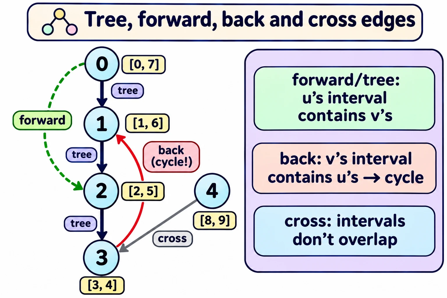
After DFS, every edge (u, v) falls into one of four types:
| Edge type | Meaning | pre/post test |
|---|---|---|
| Tree edge | DFS used it to discover v | [pre(u), post(u)] contains [pre(v), post(v)] |
| Forward edge | Goes from u down to a descendant v (not via a tree edge) | [pre(u), post(u)] contains [pre(v), post(v)] |
| Back edge | Goes from u up to an ancestor v | [pre(v), post(v)] contains [pre(u), post(u)] |
| Cross edge | Goes between two unrelated branches | The two intervals are disjoint |
Only back edges create directed cycles. So: a directed graph has a cycle if and only if DFS finds a back edge.
Worked example (we ran it). Directed graph with edges 0 → 1, 0 → 2, 1 → 2, 2 → 3, 3 → 1, 4 → 3. Run DFS from 0, then from 4 (the only vertex left unvisited).
| Vertex | 0 | 1 | 2 | 3 | 4 |
|---|---|---|---|---|---|
| pre | 0 | 1 | 2 | 3 | 8 |
| post | 7 | 6 | 5 | 4 | 9 |
| Edge | Intervals | Type |
|---|---|---|
| 0 → 1 | [0, 7] ⊇ [1, 6], used by DFS | Tree |
| 1 → 2 | [1, 6] ⊇ [2, 5], used by DFS | Tree |
| 2 → 3 | [2, 5] ⊇ [3, 4], used by DFS | Tree |
| 0 → 2 | [0, 7] ⊇ [2, 5], but 2 was found via 1 | Forward |
| 3 → 1 | [1, 6] ⊇ [3, 4] — points up to an ancestor | Back → cycle 1 → 2 → 3 → 1 |
| 4 → 3 | [8, 9] and [3, 4] don't overlap | Cross |
5. Strongly connected components (directed graphs)
Vertices i and j are strongly connected if there is a path from i to j and a path from j to i.
A directed graph splits into strongly connected components (SCCs): inside one SCC, every pair is strongly connected.
Example: in the graph above, 1 → 2 → 3 → 1, so {1, 2, 3} is one SCC. Vertex 0 can reach them but they can't reach 0, so {0} is its own SCC; likewise {4}. SCCs: {0}, {1, 2, 3}, {4}.
DFS numbering can be used to compute SCCs efficiently (and also to find articulation points — vertices whose removal disconnects the graph — and bridges — edges whose removal disconnects it). The details come later.
What's next
Directed acyclic graphs (no directed cycles) are perfect for representing dependencies — like course prerequisites. Given the prerequisites, how do we find a valid order to finish a programme? That's topological sorting (coming up).
In one line: BFS/DFS find connected components and cycles (any non-tree edge in an undirected graph); DFS pre/post numbers classify directed edges as tree/forward/back/cross, and only back edges make cycles.
Exam words: connected, connected component, isolated vertex, cycle, simple cycle, acyclic, BFS tree, DFS tree, forest, non-tree edge, pre number, post number, tree/forward/back/cross edge, strongly connected, SCC, articulation point, bridge.