
REVISION AND PRACTICE
Week 3 Quick Revision
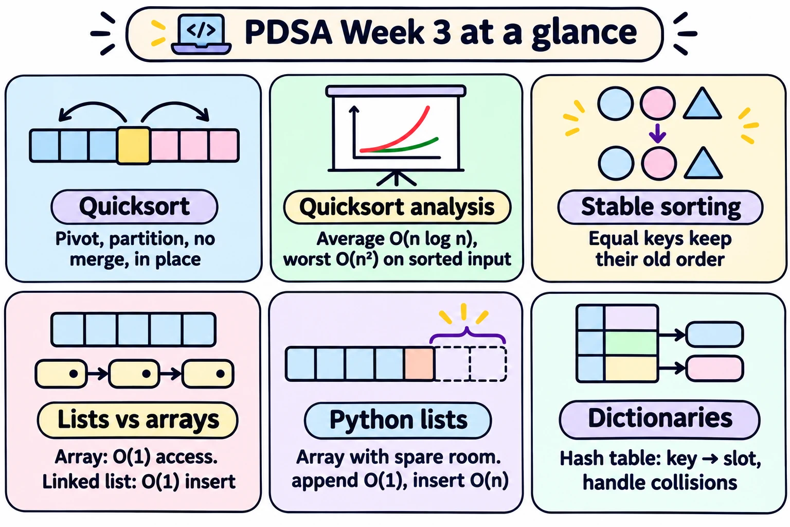
Start here Week 3 in one page: quicksort and its analysis, stable sorting and hybrids, lists vs arrays, building a linked list, how Python lists really work, and how dictionaries use hash tables.
1. Quicksort
- Pick a pivot (first element), partition into Lower (≤ pivot) and Upper (> pivot), put the pivot between them, recursively sort both sides.
- No merge step → sorts in place.
- Partition = one left-to-right pass with 4 segments: Pivot | Lower | Upper | Unclassified.
- L[i] > pivot → Upper grows (upper += 1). - L[i] ≤ pivot → swap L[i] with the first item of Upper; both markers move. - At the end: swap the pivot with the last item of Lower.
- Example: [43, 32, 22, 78, 63, 57, 91, 13] → [13, 32, 22, 43, 63, 57, 91, 78] after one partition.
2. Analysis of quicksort
| Case | Recurrence | Time |
|---|---|---|
| Pivot = median | T(n) = 2T(n/2) + n | O(n log n) |
| Pivot = min or max (sorted / reverse-sorted input!) | T(n) = T(n−1) + n | O(n²) |
| Average over all input orders | — | O(n log n) |
| Random pivot | — | O(n log n) expected for any input |
- Already sorted list = worst case for first-element pivot (we measured 4,99,500 comparisons for n = 1000).
- Iterative version: keep a to-do list of (l, r) ranges — the two parts are disjoint.
- Very fast in practice; common default library sort. (Python itself uses Timsort.)
3. Stability and choosing a sort
- Stable = equal keys keep their earlier order.
- Stable: insertion sort, merge sort with
<=. Not stable: selection sort, quicksort, merge sort with<. - Merge sort → external sorting (data on disk). Quicksort → usual default. Heapsort → another O(n log n).
- Hybrid: divide and conquer for big parts, insertion sort for small parts (n < 16).
- If moves are costly, selection sort does at most n − 1 swaps.
4. Lists vs arrays
| Operation | Array | Linked list |
|---|---|---|
| Access A[i] | O(1) | O(i) |
| Swap A[i], A[j] | O(1) | O(n) |
| Insert / delete at a known spot | O(n) | O(1) |
| Size | Fixed | Flexible |
- Array address: A[i] = start + i × slot size.
- Binary-search insert into a sorted sequence is O(n) either way.
5. Linked list in Python (class Node)
- Empty list =
Node()(value None).isempty()checksvalue == None. appendi(v): walk to the last node, attachNode(v)— O(n).insert(v)at the start: swap values with a new node, then switch links (the head can't move) — O(1).delete(v): look ahead and bypass; to delete the head's value, copy the next value in — removes the first occurrence.
6. Python lists and NumPy
- Python list = array underneath, with spare room; grows by reserving a bigger block.
append,pop()= O(1) amortised;insert,pop(0),del l[i]= O(n).- Aliasing trap:
[row, row, row]or[[0]3]3share one row. Use[[0 for i in range(3)] for j in range(3)]. - NumPy:
np.zeros(shape=(3,3)),np.array(...),np.arange(5),3A + B,np.matmul(A, B).A Bis entry-by-entry, not matrix multiplication.
7. Dictionaries = hash tables
- Array + hash function h: keys → {0, ..., n − 1}.
- Collision: two keys, same slot. A good hash function makes them rare.
- Open addressing (closed hashing): probe other slots in the same array.
- Open hashing (chaining): each slot holds a list.
- Keys must be immutable (list → TypeError: unhashable type).
- SHA-256: 256-bit industry hash, used to detect duplicate files.
Watch out — slide points to know
| Slide | Point |
|---|---|
| 3.1 partition picture | Shows Upper as 78 63 57 91; the code actually gives 63 57 91 78 — any order inside Upper is fine |
| 3.2 "quicksort is the default built-in sort" | True for many languages, but Python uses Timsort (merge + insertion hybrid, stable) |
| 3.7 "Python doubles the list size" | Good mental model; CPython actually grows by roughly 12% each time — append is still O(1) amortised |
Week 2 merge (A[i] < B[j]) | Not stable; use <= as lecture 3.4 recommends |
Practice questions
1. Partition [6, 3, 9, 1, 7, 2] with pivot 6 (lecture method). What is the list afterwards and where is 6?
i=1: 3 ≤ 6 → Lower [3]. i=2: 9 → Upper [9]. i=3: 1 ≤ 6 → swap with 9 → [6, 3, 1, 9, 7, 2]. i=4: 7 → Upper [9, 7]. i=5: 2 ≤ 6 → swap with 9 → [6, 3, 1, 2, 7, 9]. Swap pivot with last of Lower (2): [2, 3, 1, 6, 7, 9], 6 at position 3.2. How many comparisons does first-element quicksort make on a sorted list of 8 items?
7 + 6 + 5 + 4 + 3 + 2 + 1 = 28 = 8 × 7 / 2.3. Which of these are stable: selection, insertion, quicksort, merge sort with <=?
Insertion sort and merge sort with <=.4. Time to read the 1000th element: array vs linked list?
Array: O(1). Linked list: about 1000 link-follows, O(i).5. l is a Node list 2 → 4. After l.insert(1), l.appendi(5), l.delete(4), what is l?
1 → 2 → 4, then 1 → 2 → 4 → 5, then 1 → 2 → 5.6. What does this print?
<pre>m = [[0]2]2 m[0][1] = 5 print(m)</pre></summary><b>[[0, 5], [0, 5]]</b> — both rows are the same list (aliasing).</details>